Marketing Attribution: The Macro View (MMM) | Module 09

1. The Hook

I walked into Ujvi Candles holding a cup of coffee and a very confusing report.

"So," the CEO started, looking smug. "We finally launched the 'Candle Lovers' Podcast Sponsorship and those Billboards on the I-90 in Chicago. Spent $50,000. Big splash."

He turned to the screen where our SQL dashboard (the one we spent 8 weeks building) was displayed.

"Now," he asked. "Show me the rows. How many sales did the Billboards drive?"

I typed a query: SELECT * FROM marketing_touches WHERE CHANNEL = 'Billboard'.

Result: 0 rows returned.

I typed another: SELECT * FROM marketing_touches WHERE CHANNEL = 'Podcast'.

Result: 0 rows returned.

The CEO’s smile vanished. "Did we just waste $50,000?"

"No," I said. "But we hit the limit of the Pixel."

You cannot 'click' a Billboard. You cannot 'cookie' a Podcast listener.

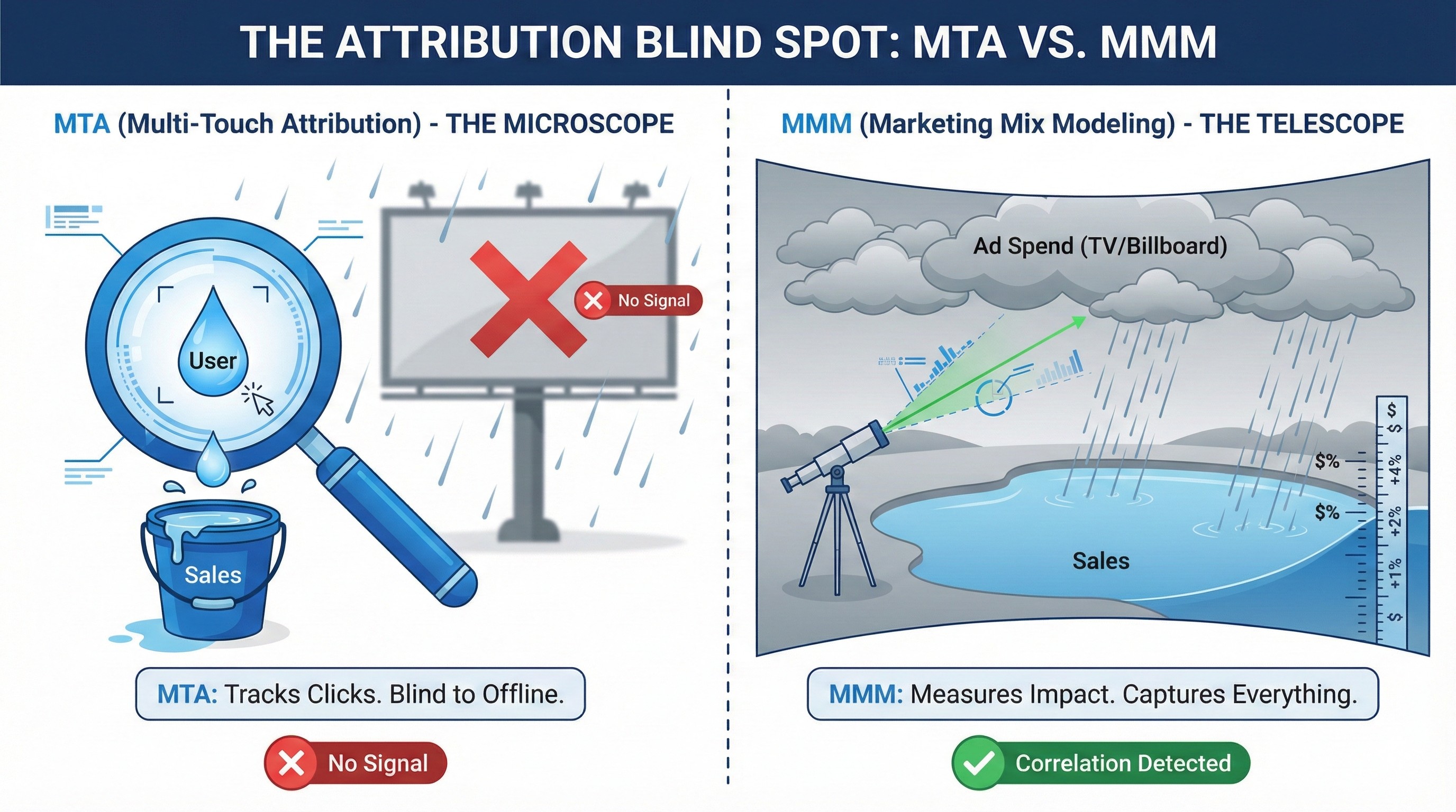
We have spent this entire series building a microscope (MTA) to track every single user. But now, Ujvi is too big for a microscope. We need a telescope. We need Marketing Mix Modeling (MMM).

2. The Concept (Top-Down vs. Bottom-Up)

Here is what I tell my clients: Stop looking at the Raindrop. Look at the Weather.

⚠️ Image Not Found
Please ensure the file is named exactly: blog 9.1.jpg

MTA (Multi-Touch Attribution): This is Bottom-Up. We track every individual raindrop (User) to see exactly which one fell into the bucket (Sale). It’s perfect for digital (Facebook, Email), but it fails when the data is invisible (TV, Radio, Word of Mouth).

MMM (Marketing Mix Modeling): This is Top-Down. We don't care about users. We look at the "Clouds" (Ad Spend) and the "Pond Level" (Total Sales).

The Logic:
We don't know who saw the Billboard. But we know this:

• Week 1: No Billboard. Sales = $10k.
• Week 2: Yes Billboard. Sales = $15k.

If the only thing that changed was the Billboard, then the Billboard drove $5k.
We stop looking at User_ID. We start looking at Date and Total_Spend.

3. The Technical Solution (Python Logic)

"We need to zoom out," I told the team. "We are going to aggregate Ujvi's data by Day."

We take our granular marketing_touches table and smash it down into a Time-Series dataset. Then, we use Ridge Regression (a fancier version of the Line of Best Fit) to find the relationship between "Activity" and "Revenue."

Step 1: The Aggregation (Python)
We convert millions of rows into a simple daily summary.

import pandas as pd
from sklearn.linear_model import Ridge

# 1. Load the Event-Level Data
df = pd.read_csv('marketing_touches.csv')
df['Date'] = pd.to_datetime(df['TOUCH_TIME']).dt.date

# 2. AGGREGATE (Zoom Out)
# Count how many times each channel was active per day
daily_activity = df.groupby(['Date', 'CHANNEL']).size().unstack(fill_value=0)

# Calculate Total Revenue per day
daily_revenue = df.groupby('Date')['ORDER_VALUE'].sum()

# 3. THE MMM DATASET
mmm_df = daily_activity.join(daily_revenue.rename('Total_Revenue'))
print(mmm_df.head())

Output: The MMM Dataset
This is what the model sees:

Step 2: The Regression (The Math)
We feed this into the model.

# 4. THE MODEL
X = mmm_df[['Facebook_Imps', 'TV_Spend', 'Billboard_Active']]
y = mmm_df['Total_Revenue']

model = Ridge(alpha=0.5)
model.fit(X, y)

# 5. THE RESULT (Coefficients)
print(f"Billboard Impact: ${model.coef_[2]:.2f} per day active")

4. The Real Data Scenario

We ran this on Ujvi's data for the last month.

The Scenario:

• Week 1: Ujvi turned OFF Facebook Ads.
  Result: Sales dropped 20%.
• Week 2: Ujvi turned ON Facebook Ads.
  Result: Sales jumped 20%.
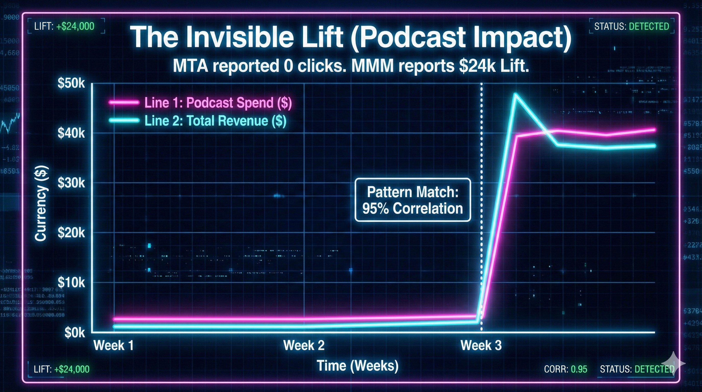
  MTA: Captures this perfectly.
• Week 3: Ujvi launched the Podcast.
  MTA Dashboard: Shows 0 clicks. 0 Conversions. Claims the Podcast is a failure.
  MMM Model: Sees that while Facebook spend stayed flat, Total Revenue jumped 10%.

⚠️ Image Not Found
Please ensure the file is named exactly: blog 9.2.jpg

The Waveform:
Visually, it looks like this. We are matching the waves.

The model calculated that for every day the Podcast was active, baseline revenue increased by $800.
MTA said the Podcast was worth $0.
MMM proved it was worth $24,000 a month.

5. The Reality Check (Adstock & Saturation)

"Okay," the CEO said. "So I should just spend infinite money on Billboards?"

"No," I warned. "Physics still applies."

MMM introduces two critical concepts that MTA ignores:

Adstock (The Echo):
If you see a TV ad today, you might not buy today. You might buy next week. The effect "decays" slowly. MMM calculates this Lag. It tells us that TV has a "Half-Life" of 2 weeks, while Facebook has a Half-Life of 1 day.

Saturation (Diminishing Returns):
The first $1,000 you spend on Billboards is powerful. The next $1,000 is good. The millionth dollar is wasted.
MMM draws the Saturation Curve. It tells Ujvi: "Stop spending on Facebook at $50k/month. You are just annoying people. Move that money to TV."

The Verdict:
MTA is for Tactics (Which creative is working? Which keyword?).
MMM is for Strategy (How much budget should go to TV vs. TikTok?).

6. Next Steps & Interaction

Ujvi now has a Micro-Model (MTA) for the daily grind and a Macro-Model (MMM) for the board meetings. But now the CEO has to make a choice. One model says spend on Facebook. The other says spend on TV.

How do we decide?

In Blog #10, we enter the final battle: MTA vs. MMM Strategy.

Over to you: Are you ready for a Cookie-less future? Do you trust a model that doesn't track users? Tell me your fears in the comments.